With a diverse and ever-expanding data warehouse or data lake with various data sources, it can become difficult to derive useful insights in a timely manner. PrestoDB is a distributed SQL query engine for big data that aims to tackle all of these problems in a federated way. It offers many connectors to the different data sources with its own query optimization and can be scaled to any number of machines to parallelize processing.

PrestoDB was born out of Facebook in 2012 after struggling with slow queries running on Apache Hive. The problem with Hive was that it would store intermediate results of its MapReduce queries on disk, which would result in a lot of I/O overhead on disk. PrestoDB, with its new architecture and in-memory engine, would significantly reduce its latencies and query speed, which in turn allows for much more interactive queries. In 2015, Netflix would show that PrestoDB was, in fact, 10 times faster than Hive and even faster in some cases.

The use cases for PrestoDB range from interactive ad hoc queries to long-running batch ETL pipelines, making it flexible for a large variety of data-driven use cases and applications.

PrestoDB resembles a massively parallel processing (MPP) system that facilitates the separation between storage and compute and allows you to scale its computing power horizontally by adding more servers. This is great for existing data storage systems and does not require migrating data from sources to run queries on them. PrestoDB is written in Java and uses the ANSI SQL specification for running queries with most features from this dialect.

In PrestoDB, you have one coordinator node and multiple worker nodes. In the case of single-node PrestoDB setups, the single node is both coordinator and worker. The coordinator node is responsible for the whole orchestration by accepting, parsing, planning, and optimizing queries. Worker nodes are responsible only for the query processing. The workers and coordinator communicate via an HTTP-based protocol on a single port.

Additionally, PrestoDB uses a discovery service that is running on the coordinator, where each worker can register and periodically send its heartbeat. This runs on the same HTTP server — including the same port.

In the following figure, you can see the full architecture in a simplified manner.

Figure 1: PrestoDB architecture

PrestoDB uses connectors to connect to the various data sources. Each connector needs to implement four service provider interfaces (SPIs):

• Metadata SPI
• Data Location SPI
• Data Statistics SPI
• Data Source SPI

These SPIs provide the interface with which PrestoDB can communicate and query data on the various data sources. The data sources are separated into connector, catalog, schema, and table concepts with the following description:

When PrestoDB executes SQL statements, they are turned into queries and then planned and executed with its query execution model using the following terminology:

 More on PrestoDB concepts: https://prestodb.io/docs/current/overview/concepts.html

Installation and Configuration

To run PrestoDB, make sure to fulfill the following prerequisites for your system:

Make sure to have Java 8 or 11 installed and make python execute python3 for the PrestoDB launcher:

sudo apt update
sudo apt install \
    python-is-python3 \
    openjdk-8-jdk-headless \
    openjdk-8-jre-headless \
    openjdk-8-jre

Download and extract the latest PrestoDB version:

wget "https://repo1.maven.org/maven2/com/facebook/presto/presto-server/0.256/presto-server-0.256.tar.gz"
tar -xzvf presto-server-0.256.tar.gz
sudo mv presto-server-0.256 /opt/presto-server
sudo chown -R $USER:$USER /opt/presto-server

Add the following lines to .bashrc file:

export PRESTO_HOME=/opt/presto-server
export PATH=$PATH:$PRESTO_HOME/bin

Then, run source ~/.bashrc for the changes to take effect. 

Single Node Configuration

PrestoDB can run both as a single node cluster or a cluster with multiple nodes. For a single node cluster, the coordinator and worker run on the same machine/instance. First, you need to create all of the configuration files for PrestoDB by creating the following folder structure:

mkdir -p /opt/presto-server/etc/catalog

The required files for a minimal setup:

• etc/node.properties
• etc/config.properties
• etc/jvm.config
• etc/log.properties

Let's have a look at each of the files above. Starting with etc/node.properties, this is its minimal configuration:

node.environment=production
node.id=ffffffff-ffff-ffff-ffff-ffffffffffff
node.data-dir=/usr/local/presto/data
plugin.dir=/opt/presto-server/plugin

Next, the configuration properties for etc/config.properties:

coordinator=true
node-scheduler.include-coordinator=true
http-server.http.port=8080
query.max-memory=5GB
query.max-memory-per-node=1GB
query.max-total-memory-per-node=2GB
discovery-server.enabled=true
discovery.uri=http://localhost:8080

The Java settings and flags can be configured in etc/jvm.config with the following minimal configuration:

-server
-Xmx16G
-XX:+UseG1GC
-XX:G1HeapRegionSize=32M
-XX:+UseGCOverheadLimit
-XX:+ExplicitGCInvokesConcurrent
-XX:+HeapDumpOnOutOfMemoryError
-XX:+ExitOnOutOfMemoryError

Finally, the logging configuration can be set in etc/log.properties:

com.facebook.presto=DEBUG

The log levels are DEBUG, INFO, WARN, and ERROR.

Multiple Nodes Configuration

The difference between multiple nodes is in etc/config.properties, which is where you define the coordinator and the discovery URL for the nodes. Additionally, you need to have a different node.id specified in each server in etc/node.properties. The configuration in etc/config.properties for the coordinator node:

coordinator=true
node-scheduler.include-coordinator=true
http-server.http.port=8080
query.max-memory=5GB
query.max-memory-per-node=1GB
query.max-total-memory-per-node=2GB
discovery-server.enabled=true
discovery.uri=http://presto-coordinator:8080

The configuration for the worker nodes:

coordinator=false
http-server.http.port=8080
query.max-memory=5GB
query.max-memory-per-node=1GB
query.max-total-memory-per-node=2GB
discovery.uri=http://presto-coordinator:8080

Troubleshooting:

• Check if each server is reachable from the other servers.
• Check if the firewall was configured properly. You need to access port 8080 or whatever port you have specified for http-server.http.port from each server to the coordinator node.
• The launcher requires Python 2.6+ or 3.5+ by calling python. Make sure to have python-is-python3 installed (sudo apt install python-is-python3).

Additional guidance: https://prestodb.io/docs/current/installation/deployment.html

For tuning your PrestoDB deployment, review the various properties: https://prestodb.io/docs/current/admin/properties.html

Launch PrestoDB

To start PrestoDB, run launcher start on each server. Below is a list of commands for the launcher:

 Once it is running, you can open http://localhost:8080 and see the cluster overview UI.

Figure 2: Presto UI

The log files can be found in data/var/log/, which are:

• data/var/log/launcher.log – Contains stdout and stderr streams of the server during initialization of the launcher.
• data/var/log/server.log – Main log file with the relevant information if the server fails during initialization. It is automatically rotated and compressed.
• data/var/log/http-request.log – HTTP request log containing all HTTP requests received by the server. It is also automatically rotated and compressed.

PrestoDB Command Line Interface

Download the PrestoDB CLI and make it executable:

wget https://repo1.maven.org/maven2/com/facebook/presto/presto-cli/0.256/presto-cli-0.256-executable.jar
mv presto-cli-0.256-executable.jar /opt/presto-server/bin/presto
chmod +x /opt/presto-server/bin/presto

Connect to PrestoDB:

presto \
    --server localhost:8080 \
    --catalog hive \
    --schema default

It is also possible to just run presto with no further settings specified. This connects to localhost:8080, and no schema or catalog would be specified.

More on the CLI: https://prestodb.io/docs/current/installation/cli.html

PrestoDB UI

The PrestoDB UI offers a large set of functionalities and insights to explore and further optimize queries. Previously, you saw the cluster-level details view, including the query list. Each query can have one of the following query states:

You can open further details on each query by clicking at the top left corner of each query item, which opens the Query Details view.

Figure 3: PrestoDB Query Details

This view includes the following sections:

• Session
• Execution
• Resource Utilization Summary
• Timeline
• Query
• Prepare Query
• Stages
• Tasks

Next, you can look at the Live Plan view, which shows the stages involved in the query.

Figure 4: PrestoDB Live Plan

You can further drill down into each stage by exploring the Stage Performance tab for each stage. 

Figure 5: PrestoDB Stage Performance

You can also see the parallelism and how the execution was done over time by checking the Splits tab.

Figure 6: PrestoDB Splits

Finally, the JSON tab will return all of the query details in a JSON. This is handy for automated evaluation of queries.

To follow along with a PrestoDB instance with a local S3 storage running on docker, feel free to use https://github.com/njanakiev/presto-minio-docker, which covers a standalone docker setup.

Connectors

PrestoDB uses a variety of connectors to access data from different data sources. In this Refcard, you will see how to access data on HDFS, S3, and PostgreSQL. More on other connectors: https://prestodb.io/docs/current/connector.html.

TPC-H and TPC-DS Connectors

TPCH (http://www.tpc.org/tpch/) and TPCDS (http://www.tpc.org/tpcds/) connectors provide a set of schemas for the TPC Benchmark™ to measure the performance of complex decision support databases. They are generally popular when running benchmarks to evaluate big data systems.

To add the tpcds connector, create the file, etc/catalog/tpcds.properties:

connector.name=tpcds

For the tpch connector, create the file, etc/catalog/tpch.properties:

connector.name=tpch 

Those connectors generate the data automatically and offer various schemas with a different number of rows for each table — and are generally great for testing queries. TPCH will be used in some of the example queries later in the Refcard.

More on these connectors:

• https://prestodb.io/docs/current/connector/tpch.html
• https://prestodb.io/docs/current/connector/tpcds.html

Hive Connector

For the Hive Connector, you need a Hive metastore running to connect either to Hadoop HDFS or an S3 storage, which is beyond the scope of this Refcard (see Additional Resources to learn more). When using HDFS, you need to configure tables with Hive. With S3, you can also specify tables for certain file types like Parquet with PrestoDB alone without creating an additional table in Hive.

The following file types are supported for the Hive Connector:

• ORC
• Parquet
• Avro
• RCFile
• SequenceFile
• JSON
• Text

Create the file, etc/cataloc/hive.properties:

connector.name=hive-hadoop2
hive.metastore.uri=thrift://HIVE_METASTORE_ENDPOINT:9083
hive.s3.path-style-access=true
hive.s3.endpoint=S3_ENDPOINT
hive.s3.aws-access-key=S3_ACCESS_KEY
hive.s3.aws-secret-key=S3_SECRET_KEY
hive.non-managed-table-writes-enabled=true
hive.s3select-pushdown.enabled=true
hive.storage-format=PARQUET

Replace S3_ENDPOINT, S3_ACCESS_KEY, and S3_SECRET_KEY with the values you specified in the metastore-site.xml or hive-site.xml configuration, as they must be identical. Then, change the HIVE_METASTORE_ENDPOINT to the endpoint of the hive metastore.

Enable S3 Select Pushdown to allow predicate pushdown by adding the property, hive.s3select-pushdown.enabled=true. If you are using multiple Hive clusters, you can add those by creating new configuration files in etc/catalog for each endpoint. This enables you to mix HDFS, AWS Glue, other S3 external object stores, and even local S3 object stores.

Create a schema to a specific bucket:

CREATE SCHEMA hive.data
WITH (location = 's3://data/')

Note that this bucket must exist beforehand. You can create it in the S3 UI or with a tool like s3cmd (https://s3tools.org/s3cmd) by running:

s3cmd mb s3://data

Now, create a new Hive table:

CREATE TABLE hive.data.example_data (
  created_at timestamp,
  user_id bigint,
  name varchar,
  country varchar
)
WITH (
  format = 'PARQUET'
);

Query the table:

SELECT created_at, user_id
FROM hive.data.example_data
LIMIT 10; 

Drop the metadata of the table (the data itself is not deleted):

DROP TABLE hive.data.example_data;

Drop a schema:

DROP SCHEMA hive.data;

More on configuration: https://prestodb.io/docs/current/connector/hive.html

PostgreSQL Connector

PostgreSQL is a popular and highly advanced, open-source RDBMS that can often be suitable for various use cases. This PrestoDB connector allows you to query and create tables in an external PostgreSQL database.

The configuration for this connector must be added to the file, etc/catalog/postgresql.properties:

connector.name=postgresql
connection-url=jdbc:postgresql://postgres-endpoint:5432/database
connection-user=username
connection-password=password

To see all schemas in PostgreSQL:

SHOW SCHEMAS FROM postgresql;

To see all tables in a schema in PostgreSQL:

SHOW TABLES FROM postgresql.public;

Further, to describe the columns in a table:

DESCRIBE postgresql.public.table_name;

To query this table:

SELECT column_1, column_2
FROM postgresql.public.table_name
WHERE column_1 IS NOT NULL
LIMIT 10;

An example of how to create a table from another table in PostgreSQL:

CREATE TABLE postgresql.public.item AS 
  SELECT i_item_id, i_item_desc
  FROM tpcds.tiny.item;

Note that CREATE TABLE by itself without AS is not supported. The same goes for these SQL statements:

• DELETE
• ALTER TABLE
• GRANT/REVOKE
• SHOW GRANTS/SHOW ROLES/SHOW ROLE GRANTS

More information: https://prestodb.io/docs/current/connector/postgresql.html.

Functions and Operators

Explore catalogs, schemas, and tables with:

PrestoDB offers a wide variety of functions and operators. You can apply logical operators with AND, OR, and NOT, as well as comparisons with <, >, and =, among others. There is a large set of commonly used mathematical functions and operators like abs(x), ceiling(x), floor(x), sqrt(x), sin(x), cos(x), tan(x), and random(), among many others. For more functions: https://prestodb.io/docs/current/functions/math.html.

The same goes for common string and date functions and operators that you might want to use. Find the full list at https://prestodb.io/docs/current/functions/string.html and https://prestodb.io/docs/current/functions/datetime.html, respectively.

When working with analytical queries, a common use case is to run aggregation over groups or whole columns. PrestoDB has many such functions that cover almost any use case. The following simple example returns the average account balance for each marketsegment in the TPCH data set:

SELECT 
  mktsegment, avg(acctbal)
FROM 
  tpch.tiny.customer
GROUP BY
  mktsegment
ORDER BY 2 DESC;

Common aggregation functions are count(), avg(), sum(x), min(x), max(x), and stddev(x), among many more advanced aggregations and statistical functions. For more: https://prestodb.io/docs/current/functions/aggregate.html

PrestoDB also offers the well-known functionality for window functions using the OVER clause. A window function uses values from one or multiple rows in a table to return a value for each row. A common example query for a rolling average over seven days:

SELECT
  orderdate,
  avg(totalprice) OVER (ORDER BY orderdate ASC ROWS 7 PRECEDING) AS rolling_average
FROM
  tpch.tiny.orders;

Another example is to calculate a sum over order priority for each row:

SELECT
  orderdate,
  totalprice,
  orderpriority,
  sum(totalprice) OVER (PARTITION BY orderpriority) 
    AS total_price_per_priority
FROM 
  tpch.tiny.orders
ORDER BY 1 ASC;

Read more about window functions: https://prestodb.io/docs/current/functions/window.html

Also, the PostGIS extension includes a large set of geospatial functions and aggregations that should be familiar to geospatial professionals coming from PostgreSQL. An example of how to aggregate data for a specific region:

SELECT 
  points.event_code,
  COUNT(points.event_id) AS cnt
FROM 
  events AS points,
  natural_earth AS countries
WHERE 
  countries.iso_a2 = 'DE'
  AND ST_Contains(
     ST_GeomFromBinary(countries.geometry), 
    ST_Point(points.lon, points.lat))
GROUP BY
  points.event_code;

A full list for the geospatial functionality: https://prestodb.io/docs/current/functions/geospatial.html

PrestoDB is quite extensive in its functionalities, and this section should serve as a quick overview of what is available. Other functions and operators include:

• Bitwise Functions
• Binary Functions and Operators
• Regular Expression Functions
• JSON Functions and Operators
• URL, IP, and HyperLogLog Functions
• Lambda Expressions
• Array and Map Functions and Operators

The complete list of functions and operators: https://prestodb.io/docs/current/functions.html

Query Optimization

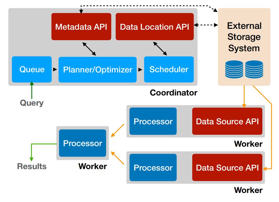
For your query to be executed on the various data sources, it requires a few steps from the initial SQL statement to the resulting query plan — where the query optimizer comes into play. After parsing the SQL statement into a syntax tree and later into a logical plan, the query optimizer takes care in creating an efficient execution strategy chosen among many possible strategies.

PrestoDB uses two optimizers. The Rule-Based Optimizer (RBO) applies filters to prune irrelevant data and uses hash joins to avoid full cartesian joins. This includes strategies such as predicate pushdown, limit pushdown, column pruning, and decorrelation. Next, it uses a Cost-Based Optimizer (CBO) continuing from the previous optimization. Here it uses statistics of the table (e.g., number of distinct values, number of null values, distributions of column data) to optimize queries and reduce I/O and network overhead.

You can see available statistics in your tables using these commands:

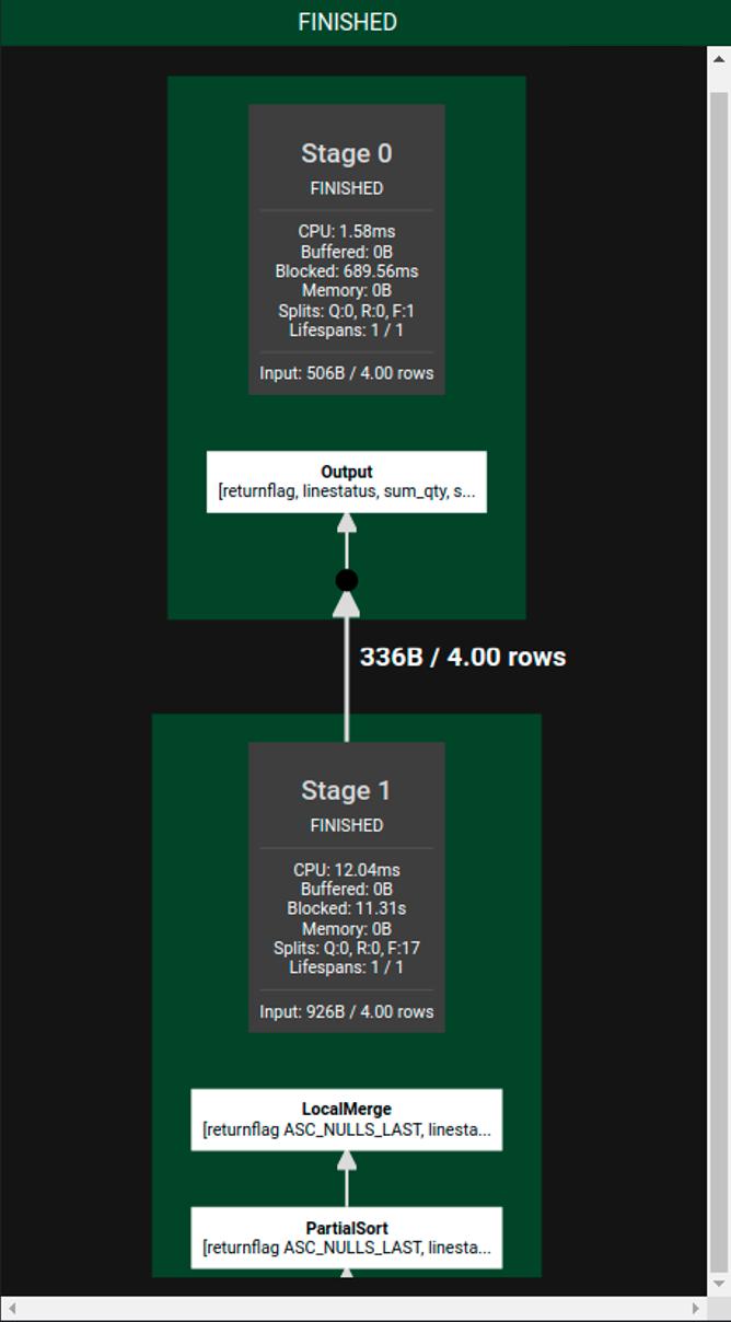
To see the cost-based analysis of a query, you can use the EXPLAIN and the EXPLAIN ANALYZE keywords:

An example of using EXPLAIN on a simple SELECT statement with the LIMIT clause, showing the calculated cost and expected number of rows:

presto> EXPLAIN SELECT mktsegment, acctbal FROM tpch.tiny.customer LIMIT 5;
 - Output[mktsegment, acctbal] => [mktsegment:varchar(10), acctbal:double]
         Estimates: {rows: 5 (70B), cpu: 21185.30, memory: 0.00, network: 70.15}
     - Limit[5] => [acctbal:double, mktsegment:varchar(10)]
             Estimates: {rows: 5 (70B), cpu: 21185.30, memory: 0.00, network: 70.15}
         - LocalExchange[SINGLE] () => [acctbal:double, mktsegment:varchar(10)]
                 Estimates: {rows: 5 (70B), cpu: 21115.15, memory: 0.00, network: 70.15}
             - RemoteStreamingExchange[GATHER] => [acctbal:double, mktsegment:varchar(10)]
                      Estimates: {rows: 5 (70B), cpu: 21115.15, memory: 0.00, network: 70.15}
                 - LimitPartial[5] => [acctbal:double, mktsegment:varchar(10)]
                         Estimates: {rows: 5 (70B), cpu: 21115.15, memory: 0.00, network: 0.00}
                     - TableScan[TableHandle {connectorId='tpch', connectorHandle='customer:sf0.01',
                          layout='Optional[customer:sf0.01]'}] => [acctbal:double, mktsegment:varchar(10)]
                              Estimates: {rows: 1500 (20.55kB), cpu: 21045.00, memory: 0.00, network: 0.00}
                              acctbal := tpch:acctbal
                              mktsegment := tpch:mktsegment

The same query with EXPLAIN ANALYZE, showing the distributed execution plan, including the duration and cost for each stage:

presto> EXPLAIN ANALYZE SELECT mktsegment, acctbal FROM tpch.tiny.customer LIMIT 5;
 Fragment 1 [SINGLE]                 
     CPU: 2.69ms, Scheduled: 13.73ms, Input: 20 rows (461B); per task: avg.: 20.00 std.dev.: 0.00, Output: 5 rows (116B)
     Output layout: [acctbal, mktsegment]
     Output partitioning: SINGLE []
     Stage Execution Strategy: UNGROUPED_EXECUTION
     - Limit[5] => [acctbal:double, mktsegment:varchar(10)]
             CPU: 0.00ns (0.00%), Scheduled: 11.00ms (5.39%), Output: 5 rows (116B)
             Input avg.: 5.00 rows, Input std.dev.: 0.00%
         - LocalExchange[SINGLE] () => [acctbal:double, mktsegment:varchar(10)]
                 CPU: 0.00ns (0.00%), Scheduled: 0.00ns (0.00%), Output: 5 rows (116B)
                 Input avg.: 1.25 rows, Input std.dev.: 387.30%
             - RemoteSource[2] => [acctbal:double, mktsegment:varchar(10)]
                     CPU: 0.00ns (0.00%), Scheduled: 0.00ns (0.00%), Output: 20 rows (461B)
                     Input avg.: 1.25 rows, Input std.dev.: 387.30%
 Fragment 2 [SOURCE]
     CPU: 20.40ms, Scheduled: 297.41ms, Input: 1500 rows (0B); per task: avg.: 1500.00 std.dev.: 0.00, Output: 20 rows (461B)
     Output layout: [acctbal, mktsegment]
     Output partitioning: SINGLE []
     Stage Execution Strategy: UNGROUPED_EXECUTION
     - LimitPartial[5] => [acctbal:double, mktsegment:varchar(10)]
             CPU: 1.00ms (5.26%), Scheduled: 160.00ms (78.43%), Output: 20 rows (461B)
             Input avg.: 375.00 rows, Input std.dev.: 0.00%
         - TableScan[TableHandle {connectorId='tpch', connectorHandle='customer:sf0.01', 
             layout='Optional[customer:sf0.01]'}, grouped = false] => [acctbal:double, mktsegment:varchar(10)]
                 CPU: 18.00ms (94.74%), Scheduled: 33.00ms (16.18%), Output: 1500 rows (33.66kB)
                 Input avg.: 375.00 rows, Input std.dev.: 0.00%
                 acctbal := tpch:acctbal
                 mktsegment := tpch:mktsegment
                 Input: 1500 rows (0B), Filtered: 0.00%

You can also add the VERBOSE option to get more detailed information and low-level statistics. For more on cost in EXPLAIN and cost-based optimizations, visit https://prestodb.io/docs/current/optimizer/cost-in-explain.html and https://prestodb.io/docs/current/optimizer/cost-based-optimizations.html, respectively.

PrestoDB is a powerful federated query engine that can bridge multiple diverse data sources and gain timely insights in an optimized way. Many companies have adopted PrestoDB in their data operations. In this Refcard, you learned about PrestoDB architecture, setup on single- and multi-node machines, and the various functionality and optimizations available. For more resources, see the following links and those throughout this Refcard.

Additional Resources

• https://prestodb.io/
• https://github.com/prestodb/presto
• https://prestodb.io/docs/current/installation/deployment.html
• https://github.com/njanakiev/presto-minio-docker
• https://research.fb.com/publications/presto-sql-on-everything/
• https://www.oreilly.com/library/view/learning-and-operating/9781492095125/