Instead of picking a single model, Ensemble Method combines multiple models in a certain way to fit the training data. Here are the two primary ways: "bagging" and "boosting." In "bagging", we take a subset of training data (pick n random sample out of N training data, with replacement) to train up each model. After multiple models are trained, we use a voting scheme to predict future data.
Random Forest is one of the most popular bagging models; in addition to selecting n training data out of N at each decision node of the tree, it randomly selects m input features from the total M input features (m ~ M^0.5). Then it learns a decision tree from that. Finally, each tree in the forest votes for the result. Here is the R code to use Random Forest:
> library(randomForest)
    #Train 100 trees, random selected attributes
    > model <- randomForest(Species~., data=iristrain, nTree=500)
    #Predict using the forest
    > prediction <- predict(model, newdata=iristest, type='class')
    > table(prediction, iristest$Species)
    > importance(model)
    MeanDecreaseGini
    Sepal.Length         7.807602
    Sepal.Width          1.677239
    Petal.Length        31.145822
    Petal.Width         38.617223
"Boosting" is another approach in Ensemble Method. Instead of sampling the input features, it samples the training data records. It puts more emphasis, though, on the training data that is wrongly predicted in previous iterations. Initially, each training data is equally weighted. At each iteration, the data that is wrongly classified will have its weight increased.
Gradient Boosting Method is one of the most popular boosting methods. It is based on incrementally adding a function that fits the residuals.
Set i = 0 at the beginning, and repeat until convergence.
- Learn a function Fi(X) to predict Y. Basically, find F that minimizes the expected(L(F(X) – Y)), where L is the lost function of the residual
- Learning another function gi(X) to predict the gradient of the above function
- Update Fi+1 = Fi + a.gi(X), where a is the learning rate
Below is Gradient-Boosted Tree using the decision tree as the learning model F. Here is the sample code in R:
> library(gbm)
    > iris2 <- iris
    > newcol = data.frame(isVersicolor=(iris2$Species=='versicolor'))
    > iris2 <- cbind(iris2, newcol)
    > iris2[45:55,]
    Sepal.Length Sepal.Width Petal.Length Petal.Width    Species isVersicolor
    45          5.1         3.8          1.9         0.4     setosa        FALSE
    46          4.8         3.0          1.4         0.3     setosa        FALSE
    47          5.1         3.8          1.6         0.2     setosa        FALSE
    48          4.6         3.2          1.4         0.2     setosa        FALSE
    49          5.3         3.7          1.5         0.2     setosa        FALSE
    50          5.0         3.3          1.4         0.2     setosa        FALSE
    51          7.0         3.2          4.7         1.4 versicolor         TRUE
    52          6.4         3.2          4.5         1.5 versicolor         TRUE
    53          6.9         3.1          4.9         1.5 versicolor         TRUE
    54          5.5         2.3          4.0         1.3 versicolor         TRUE
    55          6.5         2.8          4.6         1.5 versicolor         TRUE
    > formula <- isVersicolor ~ Sepal.Length + Sepal.Width + Petal.Length + Petal.Width
    > model <- gbm(formula, data=iris2, n.trees=1000, interaction.depth=2, distribution="bernoulli")
    Iter   TrainDeviance   ValidDeviance   StepSize   Improve
    1        1.2714         -1.#IND     0.0010    0.0008
    2        1.2705         -1.#IND     0.0010    0.0004
    3        1.2688         -1.#IND     0.0010    0.0007
    4        1.2671         -1.#IND     0.0010    0.0008
    5        1.2655         -1.#IND     0.0010    0.0008
    6        1.2639         -1.#IND     0.0010    0.0007
    7        1.2621         -1.#IND     0.0010    0.0008
    8        1.2614         -1.#IND     0.0010    0.0003
    9        1.2597         -1.#IND     0.0010    0.0008
    10        1.2580         -1.#IND     0.0010    0.0008
    100        1.1295         -1.#IND     0.0010    0.0008
    200        1.0090         -1.#IND     0.0010    0.0005
    300        0.9089         -1.#IND     0.0010    0.0005
    400        0.8241         -1.#IND     0.0010    0.0004
    500        0.7513         -1.#IND     0.0010    0.0004
    600        0.6853         -1.#IND     0.0010    0.0003
    700        0.6266         -1.#IND     0.0010    0.0003
    800        0.5755         -1.#IND     0.0010    0.0002
    900        0.5302         -1.#IND     0.0010    0.0002
    1000        0.4901         -1.#IND     0.0010    0.0002

    > prediction <- predict.gbm(model, iris2[45:55,], type="response", n.trees=1000)
    > round(prediction, 3)
    [1] 0.127 0.131 0.127 0.127 0.127 0.127 0.687 0.688 0.572 0.734 0.722
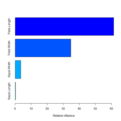
    > summary(model)
    var       rel.inf
    1 Petal.Length 61.4203761582
    2  Petal.Width 34.7557511871
    3  Sepal.Width  3.5407662531
    4 Sepal.Length  0.2831064016
The GBM R package also gave the relative importance of the input features, as shown in the bar graph.



{{ parent.title || parent.header.title}}
{{ parent.tldr }}
{{ parent.linkDescription }}
{{ parent.urlSource.name }}